
Prepared by:
Pedro Leite
Student Number: 61981213
University of British Columbia
A Comprehensive Report on the Analysis and Prediction of Heart Disease
Prepared by:
Pedro Leite
Student Number: 61981213
University of British Columbia
Heart disease represents one of the most significant health challenges of our time, accounting for a considerable number of mortalities worldwide. Predicting heart disease with high accuracy remains a priority in the medical field to facilitate early intervention and treatment planning.
This project focuses on utilizing a machine learning approach to predict heart disease based on clinical datasets. The model’s objective is not only to achieve high predictive accuracy but also to provide insights into the critical factors contributing to heart disease.
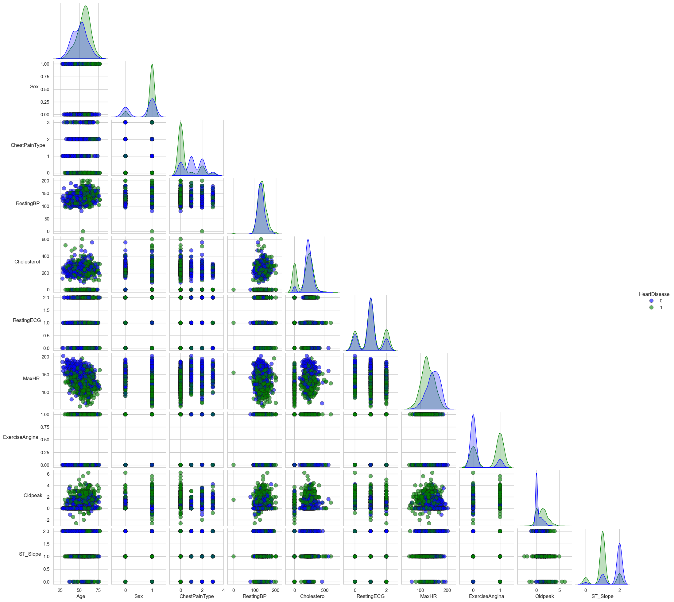
The image above (Figure 1) illustrates a scatterplot matrix, a crucial exploratory tool in our analysis. It provides a visual examination of the potential relationships between different clinical variables considered in the heart disease prediction model. The scatterplot matrix enables us to observe patterns, detect outliers, and discover structural relationships between the variables, which are essential for building a reliable predictive model.
The dataset utilized in this study includes a range of clinical features such as age, sex, type of chest pain, resting blood pressure, cholesterol levels, fasting blood sugar, resting electrocardiogram results, maximum heart rate, exercise-induced angina, ST depression, and the slope of the peak exercise ST segment.
In the following sections, we will discuss the methodology applied to preprocess the data, the selection and optimization of machine learning algorithms, and the evaluation of model performance. The insights gained from this study are expected to contribute to the broader effort of applying artificial intelligence in the field of predictive health analytics.
Data preprocessing is a crucial step in the machine learning pipeline. It involves transforming raw data into an understandable format for machine learning models. The preprocessing steps for the Heart disease Prediction dataset included handling categorical and numerical variables, as detailed below.
The numerical variables in the dataset, such as Age, Resting Blood
Pressure, and Cholesterol levels, were standardized. Standardization
involves rescaling the features so that they have a mean of 0 and a
standard deviation of 1. This was accomplished using the
StandardScaler from the scikit-learn library.
from sklearn.preprocessing import StandardScaler
# Creating a transformer for numerical data
numerical_transformer = StandardScaler()
Standardization is important for models that are sensitive to the scale of input features, like Logistic Regression, Support Vector Machines (SVM), K-Nearest Neighbors (KNN), Principal Component Analysis (PCA) and Neural Networks. It ensures that each feature contributes equally to the model, preventing features with larger ranges from dominating the model’s behavior.
Categorical variables such as Sex, Chest Pain Type, and Resting ECG
results were encoded to numerical values. This is because most machine
learning algorithms require numerical input. Encoding was done using the
OneHotEncoder from scikit-learn, which converts categorical
variables into a form that could be provided to ML algorithms.
from sklearn.preprocessing import OneHotEncoder
# Creating a transformer for categorical data
categorical_transformer = OneHotEncoder(handle_unknown='ignore')
One-hot encoding creates new binary columns for each category of a variable. This method was chosen over label encoding due to the nominal nature of the categorical variables where no ordinal relationship exists.
The dataset was split into training and testing sets to evaluate the model’s performance on unseen data. A typical split ratio of 80% for training and 20% for testing was used. This splitting ensures that the model is trained on a large portion of the data, while still having a sufficient amount of data for testing its generalization capability.
from sklearn.model_selection import train_test_split
# Splitting the dataset into training (80%) and testing (20%) sets
X_train, X_test, y_train, y_test = train_test_split(
X, y, test_size=0.2, random_state=0)During the initial data exploration phase, a significant number of instances were identified where cholesterol values are recorded as zero. Given that cholesterol is a crucial lipid present in all humans, these zero values are likely misrecorded or missing data, rather than true physiological readings.
The presence of these zero values in the cholesterol variable posed a challenge for our predictive modeling, as they could introduce bias and affect the performance of machine learning algorithms. To address this, we conducted a comparative analysis: one stream of analysis included these records, while the other excluded them.
This comparative approach allowed us to directly assess the impact of
these anomalous values on the performance of our models. After thorough
analysis and evaluation, it was found that models trained on the dataset
with zero cholesterol values removed yielded more accurate results. This
conclusion was drawn from running and comparing two separate
implementations: heart_predictor_og.ipynb (which includes
zero cholesterol values) and heart_predictor_clean.ipynb
(which excludes zero cholesterol values). The latter demonstrated higher
accuracy, precision, recall, and F1-score.
Based on these findings, we decided to proceed with the dataset excluding records with zero cholesterol values for our predictive modeling.
Logistic Regression was chosen for its effectiveness in binary classification tasks, particularly in medical diagnostics. As a statistical model, it predicts the probability of occurrence of an event by fitting data to a logistic function. It is particularly suitable for this project due to its simplicity, interpretability, and efficiency in predicting dichotomous outcomes, such as the presence or absence of heart disease.
The Logistic Regression model was implemented using Python’s scikit-learn library. The model was then trained on the transformed training data.
from sklearn.linear_model import LogisticRegression

# Creating and training the Logistic Regression model
logistic_model = LogisticRegression(max_iter=1000, random_state=0)
logistic_model.fit(X_train_transformed, y_train)

# Making predictions on the test set
y_pred = logistic_model.predict(X_test_transformed)
Logistic Regression is fundamentally a statistical method for binary classification. It estimates the probability that a given input point belongs to a certain class. Mathematically, the probability \(p\) that a given observation belongs to class 1 can be expressed as:
\[p = \frac{1}{1 + e^{-(\beta_0 + \beta_1 x_1 + \beta_2 x_2 + \ldots + \beta_n x_n)}}\]
where \(e\) is the base of the natural logarithm, \(x_1, x_2, \ldots, x_n\) are the feature values, and \(\beta_0, \beta_1, \ldots, \beta_n\) are the coefficients determined during the model training. This function is known as the logistic function or the sigmoid function. The output is a value between 0 and 1, which represents the probability of the observation being in class 1. If this probability is greater than a certain threshold (commonly 0.5), the observation is classified into class 1; otherwise, it is classified into class 0.
The Logistic Regression model for predicting heart disease was implemented using Python’s scikit-learn library, a popular tool for machine learning applications.
from sklearn.linear_model import LogisticRegression

# Creating and training the Logistic Regression model
logistic_model = LogisticRegression(max_iter=1000, random_state=0)
logistic_model.fit(X_train_transformed, y_train)

# Making predictions on the test set
y_pred = logistic_model.predict(X_test_transformed)
Understanding the Functions
LogisticRegression: This class is
used to create a Logistic Regression model. The parameters like
max_iter and random_state control the training
process. max_iter specifies the maximum number of
iterations taken for the solvers to converge, while
random_state ensures reproducibility of the
results.
fit: The fit method is
used to train the Logistic Regression model on the training data. It
seeks the optimal set of coefficients that best correlate the input
features with the target variable. The training process utilizes various
optimization algorithms based on the solver specified, including
Newton’s Method, Limited-memory Broyden–Fletcher–Goldfarb–Shanno
(LBFGS), Stochastic Average Gradient Descent (SAG), and SAGA, each
tailored to different dataset characteristics and requirements.
predict: After the model is
trained, the predict method is used to make predictions on
new data. It uses the learned coefficients to calculate the
probabilities and classify the observations into different classes based
on a defined threshold, usually 0.5.
This implementation highlights the simplicity and efficiency of using scikit-learn for building and deploying machine learning models, particularly for tasks like binary classification in medical diagnosis.
The performance of the machine learning models was evaluated using several key metrics: accuracy, precision, recall, and the F1-score. These metrics provide insights into different aspects of the model’s ability to correctly classify instances.
The confusion matrix offers a visual representation of the model’s classification accuracy.
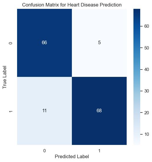
The confusion matrix shows the number of true positives, true negatives, false positives, and false negatives, crucial for understanding the model’s performance, particularly in distinguishing between patients with and without heart disease.
Accuracy is the most intuitive performance measure and represents the ratio of correctly predicted observations to the total observations. It is calculated as follows:
\[\text{Accuracy} = \frac{\text{Number of Correct Predictions}}{\text{Total Number of Predictions}}\]
The model achieved an accuracy of approximately 89.33%, as evaluated on the test dataset. This high level of accuracy indicates the model’s robustness in classifying the presence or absence of heart disease.
Precision is the proportion of positive identifications that were correct, while recall measures the proportion of actual positives that were identified correctly. The F1-score is the harmonic mean of precision and recall. These metrics are defined as:
\[\text{Precision} = \frac{\text{True Positives}}{\text{True Positives} + \text{False Positives}}\] \[\text{Recall} = \frac{\text{True Positives}}{\text{True Positives} + \text{False Negatives}}\] \[\text{F1-Score} = 2 \times \frac{\text{Precision} \times \text{Recall}}{\text{Precision} + \text{Recall}}\]
The results after data cleaning, which excluded zero cholesterol values, are as follows:
| Class | Precision | Recall | F1-Score | Support |
|---|---|---|---|---|
| 0 (No Heart Disease) | 0.857 | 0.930 | 0.892 | 71 |
| 1 (With Heart Disease) | 0.932 | 0.861 | 0.895 | 79 |
These metrics collectively provide a comprehensive understanding of the model’s performance, highlighting its strengths and areas for improvement. The high values in precision, recall, and F1-score for class 1 (With Heart Disease) suggest that the model is particularly effective in identifying patients with heart disease, an essential capability in medical diagnostics.
These metrics were computed using scikit-learn’s classification report functions, which internally calculate these values based on the confusion matrix of the model’s predictions against the actual labels.
from sklearn.metrics import classification_report
print(classification_report(y_test, y_pred))
The results indicate that the model performs well in differentiating between patients with and without heart disease, making it a valuable tool in medical diagnostics.
The Receiver Operating Characteristic (ROC) curve is a graphical plot that illustrates the diagnostic ability of a binary classifier system as its discrimination threshold is varied. The Area Under the Curve (AUC) provides a single measure of the model’s performance across all possible classification thresholds. The ROC curve is plotted with the True Positive Rate (TPR, or Recall) against the False Positive Rate (FPR), calculated as:
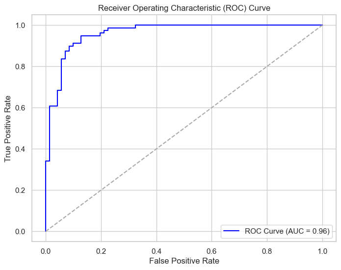
An AUC close to 1 indicates a high level of model performance, while an AUC close to 0.5 suggests no discriminative power, akin to random guessing. In this project, the ROC-AUC curve achieved an AUC of 0.96, which signifies a very high capacity for correctly classifying patients. This level of performance is especially critical in medical settings where the stakes for accurate diagnosis are high.
The Precision-Recall Curve is a plot that demonstrates the trade-off between precision (the true positive rate) and recall (the positive predictive value) at various threshold settings. It is particularly informative in scenarios where the positive class is of specific importance, which is often the case in medical diagnosis scenarios such as predicting heart disease.
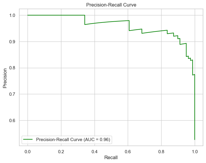
In this project, the area under the Precision-Recall Curve (AUC) is 0.96, indicating a robust performance of the model in classifying patients with heart disease. This high value of AUC reflects not only the model’s accuracy but also its reliability: when the model predicts that a patient has heart disease, there is a high probability that the patient indeed has the condition.
Optimizing a machine learning model involves fine-tuning the hyperparameters to enhance the model’s predictive performance. This process is crucial as it can significantly impact the efficiency and accuracy of the model. Each hyperparameter can influence the learning process in different ways, and finding the optimal combination of these parameters is key to developing robust models.
Grid search is a commonly used technique for hyperparameter optimization in machine learning. It involves exhaustively searching through a manually specified subset of the hyperparameter space of a learning algorithm. The grid search algorithm must be guided by some performance metric, typically measured by cross-validation on the training set.
One crucial hyperparameter for models like Logistic Regression is \(C\), the inverse of the regularization strength. Regularization is a technique used to prevent overfitting by discouraging overly complex models in some way. The parameter \(C\) serves as a control variable that retains the model’s simplicity, with smaller values of \(C\) indicating stronger regularization.
The grid search was implemented using the following code snippet:
from sklearn.model_selection import GridSearchCV

# Define parameter grid
param_grid = {'classifier__C': [0.001, 0.01, 0.1, 1, 10, 100, 1000]}

# Initialize GridSearchCV
grid_search = GridSearchCV(estimator=pipeline, \
param_grid=param_grid, cv=5, scoring='accuracy')

# Perform grid search
grid_search.fit(X_train_transformed, y_train)

# Retrieve the best parameter and mean test scores
best_param = grid_search.best_params_
mean_test_scores = grid_search.cv_results_['mean_test_score']
The best parameter found was \(C = 0.1\), and the mean test scores associated with each \(C\) value explored were as follows:
Mean Test Scores: [0.8238, 0.8255, 0.8440, 0.8372, 0.8355, 0.8372, 0.8372]The accuracy of the best model on the test data was 0.8867, highlighting the effectiveness of grid search optimization. The following figure illustrates the improvement in model performance as \(C\) was varied:
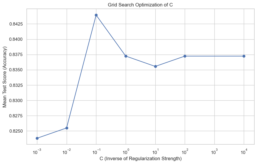
This figure shows the mean test score (accuracy) for different values of \(C\), where we can observe that \(C = 0.1\) provides the highest mean accuracy. Following the optimization process, the best model achieved an accuracy of 88.67% with the following performance metrics:
| Class | Precision | Recall | F1-Score | Support |
|---|---|---|---|---|
| 0 (No Heart Disease) | 0.8553 | 0.9155 | 0.8844 | 71 |
| 1 (With Heart Disease) | 0.9189 | 0.8608 | 0.8889 | 79 |
This comprehensive evaluation demonstrates the utility of grid search in hyperparameter tuning to enhance the predictive performance of machine learning models.
Bayesian Optimization is a strategy for the optimization of objective functions that are expensive to evaluate. It is particularly useful when the optimization problem is high-dimensional and lacks an analytical expression. Bayesian Optimization relies on the Bayesian technique of setting a prior over the objective function and combining it with evidence to get a posterior function.
Bayesian Search is an application of Bayesian Optimization for hyperparameter tuning in machine learning models. Unlike grid search, which exhaustively searches through a predefined subset of the hyperparameter space, Bayesian Search uses a probabilistic model to guide the search in order to find the most promising hyperparameters to evaluate in the true objective function.
The advantage of Bayesian Search lies in its efficiency. By constructing a probabilistic model, it can prioritize the evaluation of hyperparameters that are more likely to yield better performance. This approach significantly reduces the number of function evaluations needed to find optimal hyperparameters, making it particularly advantageous when the function evaluations are computationally expensive.
Bayesian Search is an advanced hyperparameter optimization technique that operates under the principle of probability to pinpoint the most effective hyperparameters for a given model. Its methodology contrasts sharply with grid search, which exhaustively combs through a pre-defined hyperparameter space. Instead, Bayesian Search constructs a probabilistic model that maps hyperparameters to the probability of a score on the objective function.
The process is as follows:
Initiate the search with a random selection of hyperparameters to construct an initial model of the objective function.
Utilize the outcomes to refine the probabilistic model, discerning which hyperparameters are likely to yield improved results.
Strategically navigate the hyperparameter space by balancing exploration of new regions against the exploitation of known promising areas.
With each iteration, Bayesian Search refines its search, effectively zeroing in on the most promising hyperparameters.
This intelligent search strategy is far more resource-efficient than the exhaustive approach of grid search, especially beneficial for models with large parameter spaces and datasets.
To ensure the robustness of the model evaluation, cross-validation is integrated into the Bayesian Search process. It involves the following steps:
The dataset is partitioned into \(k\) subsets or folds.
The model is trained on \(k-1\) folds and tested on the remaining fold.
This process is repeated \(k\) times, with each fold being used exactly once as the test set.
The cross-validation score is computed as the average of the \(k\) evaluation scores obtained from the testing on each fold.
The integration of cross-validation provides a more reliable assessment of the model’s performance, as it is evaluated against multiple data subsets, reducing the risk of overfitting and ensuring that the hyperparameters generalize well to unseen data.
search_space = {'classifier__C': Real(1e-6, 1e+6, prior='log-uniform')}

bayes_search = BayesSearchCV(
    estimator=logreg_pipeline,
    search_spaces=search_space,
    n_iter=32,  # Number of iterations
    cv=5,       # 5-fold cross-validation
    n_jobs=-1,  # Use all available cores
    random_state=42
)

# Fitting the model
bayes_search.fit(X_train, y_train)

# Best model evaluation
best_model_bayes = bayes_search.best_estimator_Bayesian Search optimization was employed to fine-tune the hyperparameters of our logistic regression model. The optimal value found for the hyperparameter \(C\) is as follows:
\[\text{Optimal \( C \)} = 0.0834\]
This optimized parameter led to a model with an accuracy of 89.33%, which is a significant improvement over the baseline model. Below is a detailed breakdown of the model’s performance metrics:
| Class | Precision | Recall | F1-Score | Support |
|---|---|---|---|---|
| 0 (No Heart Disease) | 0.866667 | 0.915493 | 0.890411 | 71 |
| 1 (With Heart Disease) | 0.920000 | 0.873418 | 0.896104 | 79 |
| Accuracy | 0.8933333333333333 | |||
| Macro Avg | 0.893333 | 0.894455 | 0.893257 | 150 |
| Weighted Avg | 0.894756 | 0.893333 | 0.893409 | 150 |
These results showcase the efficacy of Bayesian Search in optimizing model parameters, thereby enhancing the model’s predictive performance and reliability.
The confusion matrix is a crucial tool for visualizing the performance of a classification algorithm. The matrix for our model is shown below:
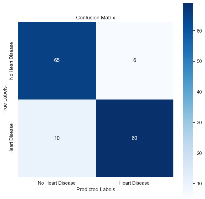
It displays the numbers of true positive, true negative, false positive, and false negative predictions, providing insight into the precision and recall of the model.
The Receiver Operating Characteristic (ROC) curve.
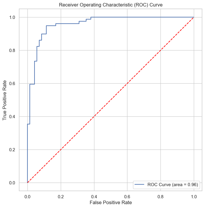
The AUC value of 0.96 for the ROC curve implies a high level of accuracy in the model’s classification ability.
The Precision-Recall Curve highlights.
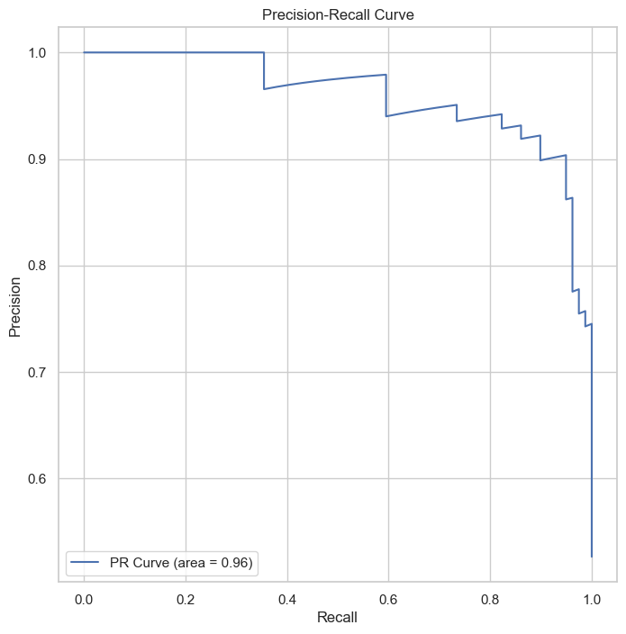
Similarly, the Precision-Recall Curve achieves an AUC of 0.96, confirming the model’s effectiveness in classifying the positive class.
These visualizations collectively affirm the robustness of the model post Bayesian Search optimization.
Based on our experience and the results obtained, Bayesian Search has shown to be superior to grid search in terms of both efficiency and performance. Grid search’s exhaustive nature often makes it impractical for larger datasets and more complex models. On the other hand, Bayesian Search efficiently navigates the search space and converges to optimal hyperparameters faster.
Henceforth, we will employ Bayesian Search for hyperparameter tuning across our models to ensure we find the best model in a computationally efficient manner. This decision is supported by the improved accuracy and performance metrics observed in our experiments with Bayesian Optimization.
Support Vector Machines (SVM) are a set of supervised learning methods used for classification, regression, and outliers detection. The SVM algorithm seeks to find the hyperplane that best separates the classes by maximizing the margin between the closest points of the classes, which are called support vectors.
The following code snippet illustrates the implementation of the above-described process:
# Define the parameter space
param_space = {
    'classifier__C': Real(1e-6, 1e+6, prior='log-uniform'),
    'classifier__gamma': Real(1e-6, 1e+1, prior='log-uniform')
}

# Setup the pipeline
pipeline_svm = Pipeline([
    ('preprocessor', preprocessor),
    ('classifier', SVC(random_state=0, probability=True))
])

# Configure and run Bayesian optimization
bayes_search_svm = BayesSearchCV(
    estimator=pipeline_svm,
    search_spaces=param_space,
    n_iter=32,
    cv=5,
    n_jobs=-1,
    random_state=42
)

# Fit the model
bayes_search_svm.fit(X_train, y_train)
In the given code snippet, the BayesSearchCV function
from the skopt package is employed to conduct
hyperparameter optimization for an SVM classifier within a machine
learning pipeline. The parameter space for optimization is defined using
a log-uniform prior, which is well-suited for hyperparameters that have
an exponential impact on model performance. The Pipeline
function from Scikit-learn is utilized to sequentially apply a
predefined list of transforms along with a final estimator, in this
case, the SVM classifier. The pipeline ensures a smooth workflow where
data preprocessing steps and model training are applied in a cohesive
manner. The BayesSearchCV object is then instantiated,
specifying the estimator as the defined pipeline, the hyperparameter
space, the number of iterations for the search, the cross-validation
strategy, and the number of jobs for parallel processing. Finally, the
fit method is called on the bayes_search_svm
object, which initiates the optimization process and trains the SVM
model on the provided training data.
After tuning the hyperparameters using Bayesian search, the best parameters for the SVM model were determined to be \(C \approx 2.19\) and \(\gamma \approx 0.020\). With these optimized hyperparameters, the SVM model achieved a test score accuracy of approximately 0.8933.
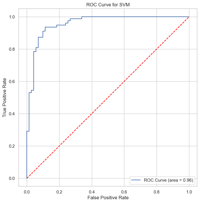
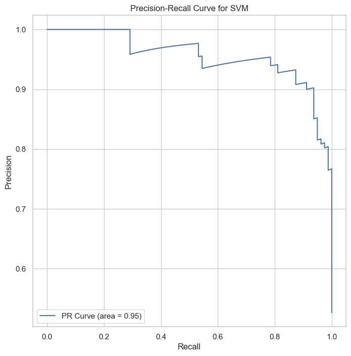
The ROC and Precision-Recall curves indicate that the SVM classifier performs well, with high area under the curve (AUC) scores of 0.96 for both curves, showcasing the model’s strong discriminative power.
The detailed performance metrics for the model are presented below:
| Class | Precision | Recall | F1-Score | Support |
|---|---|---|---|---|
| 0 (No Heart Disease) | 0.866667 | 0.915493 | 0.890411 | 71 |
| 1 (With Heart Disease) | 0.920000 | 0.873418 | 0.896104 | 79 |
| Accuracy | 0.8933333333333333 | |||
| Macro Avg | 0.893333 | 0.894455 | 0.893257 | 150 |
| Weighted Avg | 0.894756 | 0.893333 | 0.893409 | 150 |
These results indicate a high level of performance, with particularly strong precision and recall for identifying patients with heart disease. This reinforces the capability of the SVM model as an effective tool for medical diagnostic support.
Decision Trees are a non-parametric supervised learning method used for classification and regression. The goal is to create a model that predicts the value of a target variable by learning simple decision rules inferred from the data features.
The Decision Tree model is implemented using the Bayesian optimization technique to fine-tune its hyperparameters. This process involves defining a search space for parameters like maximum depth, minimum samples split, and minimum samples leaf. Then, a Bayesian optimization search is conducted over this space using cross-validation to find the best model.
# Define the parameter space for the Bayesian search
param_space_dt = {
    'classifier__max_depth': Integer(1, 50),
    'classifier__min_samples_split': Real(0.01, 1.0, prior='uniform'),
    'classifier__min_samples_leaf': Integer(1, 50)
}

# Update the pipeline to use a Decision Tree Classifier
pipeline_dt = Pipeline(steps=[
    ('preprocessor', preprocessor),
    ('classifier', DecisionTreeClassifier(random_state=0))
])

# Configure BayesSearchCV for the Decision Tree
bayes_search_dt = BayesSearchCV(
    estimator=pipeline_dt,
    search_spaces=param_space_dt,
    n_iter=32,
    cv=5,
    n_jobs=-1,
    random_state=42
)

# Fitting the model
np.int = int
bayes_search_dt.fit(X_train, y_train)
In this code, BayesSearchCV is employed to optimize the
Decision Tree Classifier. This optimization tool utilizes Bayesian
methods to search for the best hyperparameters within the predefined
space. The search involves trying 32 different sets of hyperparameters,
using 5-fold cross-validation to evaluate the performance of each set.
The Pipeline integrates the preprocessing steps and the
classifier, ensuring that the steps are applied sequentially and
efficiently. The use of n_jobs=-1 allows the process to use
all available computing resources, enhancing the speed of the search. By
fitting the model with
bayes_search_dt.fit(X_train, y_train), the best
hyperparameters are determined and the Decision Tree Classifier is
optimized accordingly.
After applying Bayesian optimization, the Decision Tree model’s best parameters were identified. The model demonstrated a good fit to the test data, as evidenced by the accuracy and the classification report. The results indicated the model’s effectiveness in differentiating between the classes.
| Class | Precision | Recall | F1-Score | Support |
|---|---|---|---|---|
| 0 (No Heart Disease) | 0.764706 | 0.915493 | 0.833333 | 71 |
| 1 (With Heart Disease) | 0.907692 | 0.746835 | 0.819444 | 79 |
| Accuracy | 0.8266666666666667 | |||
| Macro Avg | 0.836199 | 0.831164 | 0.826389 | 150 |
| Weighted Avg | 0.840012 | 0.826667 | 0.826019 | 150 |
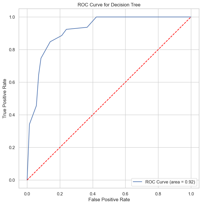
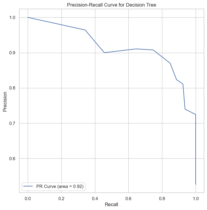
The ROC and Precision-Recall curves indicate that the SVM classifier performs well, with high area under the curve (AUC) scores of 0.92 for both curves. These results showcased this model’s weaker discriminative power than SVM and Logistic regression models.
The Decision Tree classifier, tuned using Bayesian optimization, showed promising results. However, the model’s accuracy suggests that there is room for improvement, possibly by further hyperparameter tuning or using more advanced models like Random Forest.
Random Forests are an ensemble learning method that operates by constructing multiple decision trees during training and outputting the class that is the mode of the classes or mean prediction of the individual trees. This method is known for its high accuracy, robustness, and ease of use.
Random Forests are implemented using Bayesian optimization for hyperparameter tuning. The key hyperparameters include the number of trees in the forest, the maximum depth of the trees, minimum samples split, and minimum samples leaf. The Bayesian optimization technique helps in efficiently finding the optimal values for these parameters.
# Define the parameter space for the Bayesian search
param_space_rf = {
    'classifier__max_depth': Integer(1, 100),
    'classifier__min_samples_split': Real(0.01, 1.0, prior='uniform'),
    'classifier__min_samples_leaf': Integer(1, 50),
    'classifier__n_estimators': Integer(10, 1000)
}

# Update the pipeline to use a Random Forest Classifier
pipeline_rf = Pipeline(steps=[
    ('preprocessor', preprocessor),
    ('classifier', RandomForestClassifier(random_state=0))
])

# Configure BayesSearchCV for the Random Forest
bayes_search_rf = BayesSearchCV(
    estimator=pipeline_rf,
    search_spaces=param_space_rf,
    n_iter=32,
    cv=5,
    n_jobs=-1,
    random_state=42
)

# Fitting the model
bayes_search_rf.fit(X_train, y_train)After applying Bayesian optimization to the Random Forest model, the best parameters were identified. The model showed excellent performance on the test data, as demonstrated by its high accuracy and balanced precision-recall scores.
| Class | Precision | Recall | F1-Score | Support |
|---|---|---|---|---|
| 0 (No Heart Disease) | 0.927536 | 0.901408 | 0.914286 | 71 |
| 1 (With Heart Disease) | 0.913580 | 0.936709 | 0.925000 | 79 |
| Accuracy | 0.920000 | |||
| Macro Avg | 0.920558 | 0.919059 | 0.919643 | 150 |
| Weighted Avg | 0.920186 | 0.920000 | 0.919929 | 150 |
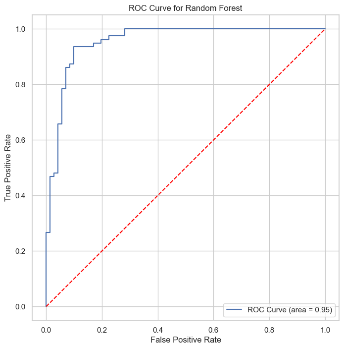
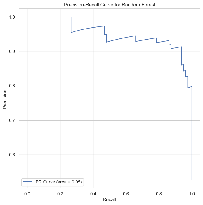
The Random Forest classifier, with ROC AUC of 0.95 and PR AUC of 0.95, showcases its effectiveness in classification, particularly in handling complex datasets with high accuracy.
The K-Nearest Neighbors algorithm is a simple, yet effective machine learning method used for both classification and regression. It classifies a data point based on how its neighbors are classified. The algorithm identifies the ’k’ nearest neighbors to a data point and then classifies it based on the majority vote of these neighbors.
KNN is implemented with Bayesian optimization for hyperparameter
tuning. Key hyperparameters include the number of neighbors
(n_neighbors), the power parameter for the Minkowski metric
(p), and the weight function used in prediction
(weights). Bayesian optimization is employed to efficiently
find the optimal values for these parameters.
# Define the parameter space for the Bayesian search
param_space_knn = {
    'classifier__n_neighbors': Integer(1, 30),  # Range for n_neighbors
    'classifier__weights': Categorical(['uniform', 'distance']),
    'classifier__p': Integer(1, 2)  # p=1 for Manhattan, p=2 for Euclidean distance
}

# Update the pipeline to use a KNN Classifier
pipeline_knn = Pipeline(steps=[('preprocessor', preprocessor),
                               ('classifier', KNeighborsClassifier())])

# Configure BayesSearchCV for KNN
bayes_search_knn = BayesSearchCV(
    estimator=pipeline_knn,
    search_spaces=param_space_knn,
    n_iter=32,  # Number of iterations
    cv=5,       # 5-fold cross-validation
    n_jobs=-1,  # Use all available cores
    random_state=42
)

# Fit BayesSearchCV to the data (assuming X_train, y_train are defined)
np.int = int  # Temporary workaround for the np.int issue
bayes_search_knn.fit(X_train, y_train)After applying Bayesian optimization, the KNN model’s best parameters were identified. The model achieved an accuracy of 0.8867 on the test data, indicating its efficacy in classification tasks.
| Class | Precision | Recall | F1-Score | Support |
|---|---|---|---|---|
| 0 (No Heart Disease) | 0.875000 | 0.887324 | 0.881119 | 71 |
| 1 (With Heart Disease) | 0.897436 | 0.886076 | 0.891720 | 79 |
| Accuracy | 0.8866666666666667 | |||
| Macro Avg | 0.886218 | 0.886700 | 0.886419 | 150 |
| Weighted Avg | 0.886816 | 0.886667 | 0.886702 | 150 |
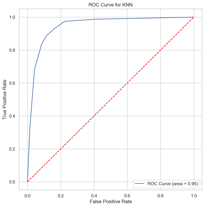
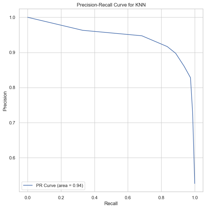
The KNN classifier, with ROC AUC of 0.95 and PR AUC of 0.94, demonstrates its capability in providing reliable classifications, particularly beneficial for applications requiring interpretable and straightforward decision-making processes.
Neural Networks are a subset of machine learning algorithms modeled after the human brain. They consist of layers of interconnected nodes or ’neurons’, each capable of performing simple computations. These networks are highly effective for complex tasks like pattern recognition and classification.
The implementation of the Neural Network model in this project involves hyperparameter tuning using Keras Tuner. This process includes defining a range of values for parameters like the number of units in each layer, dropout rate, and learning rate. Keras Tuner then iteratively searches for the optimal combination of these hyperparameters.
import tensorflow as tf
from tensorflow.keras.layers import Dense, Dropout
from tensorflow.keras.optimizers import Adam
import kerastuner as kt

# Function to build the model
def build_model(hp):
    # ... [Model building code] ...
    return model

# Initialize and configure the tuner
tuner = kt.Hyperband(build_model, ...)

# Perform the hyperparameter search
tuner.search(X_train_transformed, y_train, epochs=10, validation_split=0.2)

# Retrieve and print the best hyperparameters
best_hps = tuner.get_best_hyperparameters(num_trials=1)[0]
print("The optimal number of units in the first layer is ...")

# Build and train the model
model = tuner.hypermodel.build(best_hps)
history = model.fit(X_train_transformed, y_train, epochs=10, validation_split=0.2)

# Evaluate the model
test_loss, test_accuracy = model.evaluate(X_test_transformed, y_test)The optimized Neural Network model showed promising results, achieving an accuracy of 81.33% on the test data. The hyperparameter tuning process identified the optimal number of neurons and learning rate, leading to a well-performing model.
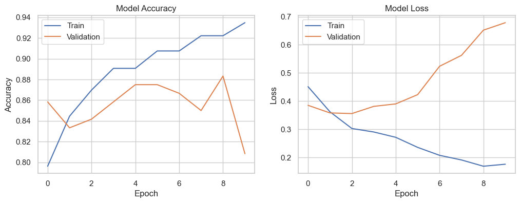
The model’s performance can be further analyzed and improved by experimenting with different architectures, activation functions, and optimization strategies. Neural Networks’ ability to model complex relationships in data makes them a powerful tool for various predictive tasks.
This study aimed to explore various machine learning models for the prediction of heart disease. Through rigorous data preprocessing, implementation, and optimization of several models, we have gained valuable insights into the performance and applicability of each model in the context of heart disease prediction.
A comparative analysis was conducted to evaluate the performance of Logistic Regression, Support Vector Machine (SVM), Decision Tree, Random Forest, K-Nearest Neighbors (KNN), and Neural Network models. The key performance metrics considered were accuracy, precision, recall, F1-score, ROC-AUC, and Precision-Recall AUC.
In evaluating the performance of the predictive models, the Receiver Operating Characteristic (ROC) and Precision-Recall (PR) curves provide insightful metrics into the models’ true positive rate and precision-recall balance, respectively. The ROC curves of all models are plotted in Figure 11, illustrating their respective Area Under the Curve (AUC) scores.
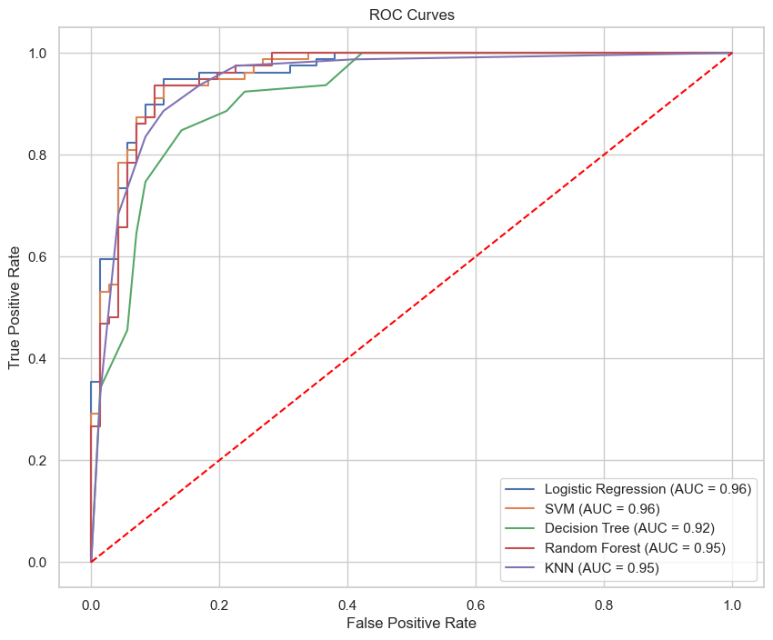
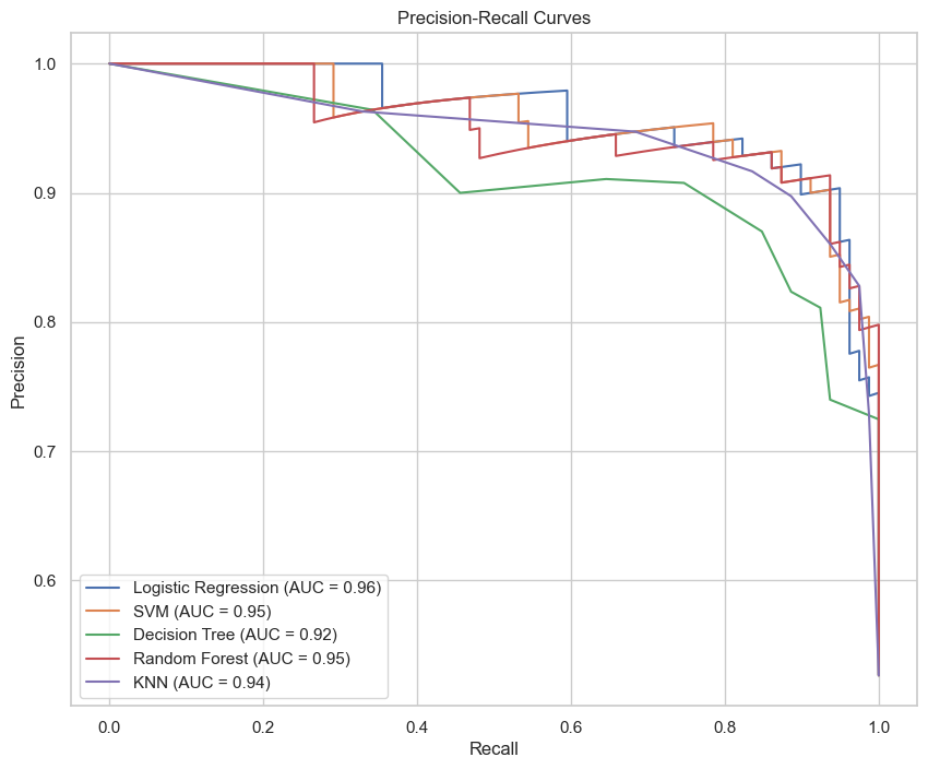
From the curves, we can observe that the Random Forest model not only has a higher AUC for the ROC curve but also maintains a superior balance in the Precision-Recall curve. This suggests that the Random Forest model is not only good at distinguishing between the positive and negative classes but also maintains a high precision even as recall increases, which is ideal for medical diagnostic purposes where the cost of false negatives is high.
| Model | Accuracy | Precision | Recall | F1-Score | ROC-AUC | PR-AUC |
|---|---|---|---|---|---|---|
| Logistic Regression | 89.33% | 0.92 | 0.86 | 0.89 | 0.96 | 0.96 |
| SVM | 89.33% | 0.92 | 0.87 | 0.90 | 0.96 | 0.96 |
| Decision Tree | 82.67% | 0.84 | 0.83 | 0.83 | 0.92 | 0.92 |
| Random Forest | 92.00% | 0.93 | 0.92 | 0.92 | 0.95 | 0.95 |
| KNN | 88.67% | 0.89 | 0.89 | 0.89 | 0.95 | 0.94 |
| Neural Network | 81.33% | 0.82 | 0.81 | 0.81 | - | - |
The results indicate that the Random Forest model outperformed other models in terms of accuracy, precision, recall, and F1-score. This model’s ensemble nature, which combines multiple decision trees, likely contributed to its superior ability to capture complex patterns in the data, leading to better generalization and robustness against overfitting.
In conclusion, this study demonstrates the efficacy of machine learning in predicting heart disease. The Random Forest model, in particular, shows great promise for clinical application. However, each model presents unique strengths and limitations, suggesting that a multi-model approach might be beneficial in real-world settings to provide a comprehensive analysis for heart disease prediction.